Swin Transformer: Hierarchical Vision Transformer using Shifted Windows
Overview
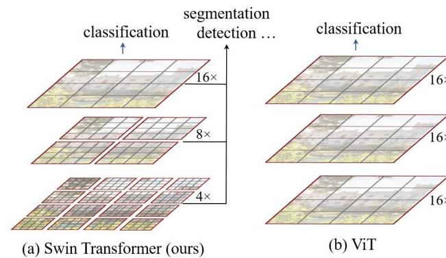
Vision Transformers (ViT) demonstrated that pure transformer architectures could match or exceed CNNs on image classification, but ViT's design introduced two fundamental limitations for general-purpose vision: it operates at a single low resolution (16x downsampled patches throughout), making it unsuitable for dense prediction tasks that require multi-scale features; and its global self-attention has quadratic computational complexity with respect to image size, making it impractical for high-resolution inputs. These limitations confined ViT primarily to classification and prevented it from serving as a general backbone for detection, segmentation, and other dense tasks.
Swin Transformer addresses both problems through two key design choices: a hierarchical feature pyramid that produces representations at multiple resolutions (like a CNN backbone), and shifted window self-attention that computes attention within local windows for linear complexity while using window shifting between layers to enable cross-window information flow. The hierarchical structure is built by progressively merging neighboring patches at each stage (analogous to pooling in CNNs), producing feature maps at 4x, 8x, 16x, and 32x downsampling -- exactly the multi-scale structure that FPN-based detectors and segmentation heads expect.
The results established Swin Transformer as the first general-purpose vision transformer backbone. It achieved 87.3% top-1 accuracy on ImageNet-1K (with ImageNet-22K pretraining), 58.7 box AP / 51.1 mask AP on COCO object detection (surpassing prior art by +2.7 box AP / +2.6 mask AP), and 53.5 mIoU on ADE20K semantic segmentation. These results represented substantial improvements over both CNN and prior transformer backbones across all three tasks, demonstrating that transformers could serve as drop-in replacements for ResNet/ResNeXt in existing detection and segmentation frameworks.
Key Contributions
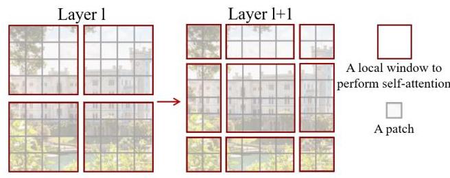
- Shifted window self-attention mechanism: Computes self-attention within non-overlapping local windows (W-MSA), then shifts the window partition by half the window size in alternating layers (SW-MSA), creating cross-window connections at effectively zero additional cost. This achieves linear computational complexity O(n) with respect to image size, compared to O(n^2) for global self-attention.
- Hierarchical feature pyramid via patch merging: Produces multi-scale feature maps (C, 2C, 4C, 8C channels at 1/4, 1/8, 1/16, 1/32 resolution) by concatenating and linearly projecting 2x2 groups of neighboring patches between stages, enabling direct compatibility with FPN, UPerNet, and other multi-scale architectures.
- Efficient cyclic shift implementation: Instead of naively computing attention for multiple smaller shifted windows (which would be irregular and slow), uses cyclic shifting of the feature map combined with attention masking. This maintains batched computation within the same window size while correctly restricting attention to non-shifted neighbors.
- Relative position bias: Replaces absolute position embeddings with a learnable relative position bias added to each attention head, parameterized by relative offsets. This provides +0.8% top-1 accuracy on ImageNet over absolute position embeddings (+1.2% over no position embedding at all) and transfers better across varying input resolutions.
- General-purpose backbone demonstration: First transformer architecture to serve as a drop-in backbone for detection (Cascade Mask R-CNN, HTC++), segmentation (UPerNet), and classification simultaneously, establishing the template that subsequent architectures (Swin V2, CSWin, Focal Transformer) followed.
Architecture / Method
                         Swin Transformer Hierarchical Architecture

  Input Image (H x W x 3)
        │
        ▼
  ┌──────────────────────┐
  │  Patch Partition 4x4  │  ──►  H/4 x W/4 tokens, dim C
  │  + Linear Embedding   │
  └──────────┬───────────┘
             │
             ▼
  ┌──────────────────────┐
  │  Stage 1: Swin Blocks │  ──►  H/4 x W/4,  C     (1/4 res)
  │  [W-MSA ─► SW-MSA]x2  │
  └──────────┬───────────┘
             │  Patch Merging (2x2 concat ──► linear)
             ▼
  ┌──────────────────────┐
  │  Stage 2: Swin Blocks │  ──►  H/8 x W/8,  2C    (1/8 res)
  │  [W-MSA ─► SW-MSA]x2  │
  └──────────┬───────────┘
             │  Patch Merging
             ▼
  ┌──────────────────────┐
  │  Stage 3: Swin Blocks │  ──►  H/16 x W/16, 4C   (1/16 res)
  │  [W-MSA ─► SW-MSA]xN  │
  └──────────┬───────────┘
             │  Patch Merging
             ▼
  ┌──────────────────────┐
  │  Stage 4: Swin Blocks │  ──►  H/32 x W/32, 8C   (1/32 res)
  │  [W-MSA ─► SW-MSA]x2  │
  └──────────────────────┘

  Each Swin Block:
  ┌─────────────────────────────────────────┐
  │  Input ─► LN ─► W-MSA  ─► + (residual) │
  │        ─► LN ─► MLP    ─► + (residual) │
  │        ─► LN ─► SW-MSA ─► + (residual) │
  │        ─► LN ─► MLP    ─► + (residual) │
  └─────────────────────────────────────────┘
Hierarchical Design
The architecture processes an input image through four stages, each operating at a different spatial resolution:
- Patch Partition + Linear Embedding (Stage 1): The input image (H x W x 3) is split into non-overlapping 4x4 patches, each flattened and projected to dimension C via a linear layer. This produces H/4 x W/4 tokens of dimension C.
- Stage 2: Patch merging concatenates 2x2 groups of adjacent tokens (4C channels), then a linear layer reduces to 2C. Resolution becomes H/8 x W/8.
- Stage 3: Same patch merging process, producing H/16 x W/16 tokens of dimension 4C.
- Stage 4: Final merging to H/32 x W/32 tokens of dimension 8C.
Each stage contains a stack of Swin Transformer blocks. The standard model variants are:
| Variant | C | Layers per stage | Heads per stage | Params | FLOPs |
|---|---|---|---|---|---|
| Swin-T | 96 | 2, 2, 6, 2 | 3, 6, 12, 24 | 29M | 4.5G |
| Swin-S | 96 | 2, 2, 18, 2 | 3, 6, 12, 24 | 50M | 8.7G |
| Swin-B | 128 | 2, 2, 18, 2 | 4, 8, 16, 32 | 88M | 15.4G |
| Swin-L | 192 | 2, 2, 18, 2 | 6, 12, 24, 48 | 197M | 34.5G |
Shifted Window Self-Attention
Each Swin Transformer block consists of a window-based multi-head self-attention (W-MSA) or shifted-window multi-head self-attention (SW-MSA), followed by a 2-layer MLP with GELU activation. LayerNorm is applied before each module, and residual connections after each:
z_l   = W-MSA(LN(z_{l-1})) + z_{l-1}
z_l   = MLP(LN(z_l)) + z_l
z_{l+1} = SW-MSA(LN(z_l)) + z_l
z_{l+1} = MLP(LN(z_{l+1})) + z_{l+1}
W-MSA partitions the feature map into non-overlapping M x M windows (default M=7) and computes standard multi-head self-attention independently within each window. Complexity per window: O(M^2 * M^2) = O(M^4). Total complexity for an h x w feature map: O(h * w * M^2), which is linear in image size.
SW-MSA shifts the window partition by (floor(M/2), floor(M/2)) pixels, so that the boundaries of the previous partitioning fall in the middle of new windows. This allows tokens at the edges of the original windows to attend to each other.
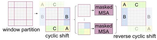
Efficient Cyclic Shift
Rather than padding or handling variable-size windows, the implementation cyclically shifts the feature map by (floor(M/2), floor(M/2)) before partitioning into regular M x M windows, then applies masking within the attention computation to prevent tokens from different original regions from attending to each other. After attention, the feature map is shifted back. This keeps all windows the same size for efficient batched computation.
Relative Position Bias
Instead of absolute position embeddings, each attention head adds a bias term B from a learnable table indexed by the relative position between tokens:
Attention(Q, K, V) = SoftMax(QK^T / sqrt(d) + B) V
The bias table has shape (2M-1) x (2M-1) for each head, covering all possible relative positions within an M x M window. Relative position bias is significantly more effective than absolute embeddings (+0.8% top-1 on ImageNet over absolute pos., +1.2% over no position embedding) and allows the model to generalize across different input resolutions at fine-tuning time by interpolating the bias table.
Results
ImageNet-1K Classification
| Method | Pretrain | Resolution | Top-1 Acc | Params | FLOPs |
|---|---|---|---|---|---|
| ResNet-50 | IN-1K | 224 | 76.2 | 25M | 4.1G |
| DeiT-S | IN-1K | 224 | 79.8 | 22M | 4.6G |
| Swin-T | IN-1K | 224 | 81.3 | 29M | 4.5G |
| Swin-S | IN-1K | 224 | 83.0 | 50M | 8.7G |
| Swin-B | IN-1K | 224 | 83.5 | 88M | 15.4G |
| ViT-B/16 | IN-21K | 384 | 84.0 | 86M | 55.5G |
| Swin-B | IN-22K | 384 | 86.4 | 88M | 47.0G |
| Swin-L | IN-22K | 384 | 87.3 | 197M | 103.9G |
COCO Object Detection (Cascade Mask R-CNN, 3x schedule)
| Backbone | box AP | mask AP | Params | FLOPs |
|---|---|---|---|---|
| ResNet-50 | 46.3 | 40.1 | 82M | 739G |
| X101-64 | 48.3 | 41.7 | 140M | 972G |
| Swin-T | 50.4 | 43.7 | 86M | 745G |
| Swin-S | 51.9 | 45.0 | 107M | 838G |
| Swin-B | 51.9 | 45.0 | 145M | 982G |
| Swin-L (HTC++) | 58.7 | 51.1 | 284M | - |
ADE20K Semantic Segmentation (UPerNet)
| Backbone | mIoU (single-scale) | mIoU (multi-scale) | Params | FLOPs |
|---|---|---|---|---|
| ResNet-101 | 44.9 | - | 86M | 1029G |
| DeiT-S + MLN | 43.8 | - | 58M | 1217G |
| Swin-T | 44.5 | 45.8 | 60M | 945G |
| Swin-S | 47.6 | 49.5 | 81M | 1038G |
| Swin-L | 52.1 | 53.5 | 234M | 2468G |
Key Ablation Results
| Ablation | Top-1 Acc | Delta |
|---|---|---|
| Swin-T (shifted windows) | 81.3 | baseline |
| No shifting (W-MSA only) | 80.2 | -1.1 |
| No position embedding | 80.1 | -1.2 |
| Absolute position embedding | 80.5 | -0.8 vs rel. pos. |
| Relative position bias | 81.3 | +0.8 vs abs. pos., +1.2 vs no pos. |
| Sliding window (3x3) | 81.4 | +0.1 but 40.8x slower |
The shifted window mechanism provides +1.1% over non-shifted windows at no computational cost increase. The sliding window approach achieves only marginal additional accuracy (+0.1%) while being 40.8x slower, validating that shifted windows capture nearly all cross-window benefits at a fraction of the cost.
Limitations & Open Questions
- Fixed window size: The M=7 window size is a hyperparameter that may not be optimal for all resolutions or tasks. Larger windows improve receptive field but increase per-window quadratic cost.
- Shift pattern rigidity: The fixed half-window shift pattern is simple but may miss long-range dependencies that require more than 2 layers to propagate across the image.
- Resolution transfer: While relative position bias helps, transferring from 224 to 384+ resolution still requires bias interpolation and careful fine-tuning.
- Dense prediction overhead: Despite hierarchical design, the patch merging operations add non-trivial overhead compared to simple strided convolutions in CNNs.
- Subsequent work: Swin V2 (2022) addressed several of these limitations with log-spaced continuous position bias, residual post-normalization for training stability at larger scales, and SimMIM self-supervised pretraining.
Connections
Related papers in the wiki: - Attention Is All You Need -- the original transformer architecture that Swin adapts for vision - An Image Is Worth 16X16 Words Transformers For Image Recognition At Scale -- ViT, the direct predecessor; Swin solves ViT's single-scale and quadratic complexity limitations - Deep Residual Learning For Image Recognition -- ResNet, the CNN backbone that Swin replaces as the standard vision backbone - Imagenet Classification With Deep Convolutional Neural Networks -- AlexNet, the original CNN backbone paradigm that hierarchical vision transformers supersede - Bevformer Learning Birds Eye View Representation From Multi Camera Images Via Spatiotemporal Transformers -- uses Swin-style hierarchical features as backbone for BEV perception - Learning Transferable Visual Models From Natural Language Supervision -- CLIP, contemporary vision-language model that also demonstrated transformer backbones for vision - Perception -- Swin Transformer became a standard backbone for driving perception systems