Deep Residual Learning for Image Recognition

Citation

He, Zhang, Ren, Sun (Microsoft Research), CVPR, 2016.

Canonical link

Paper

Overview

Deep Residual Learning introduces skip connections that add the input identity to learned residual functions, solving the degradation problem that prevented training of very deep networks. This simple modification enabled networks with 100+ layers to train successfully, achieving state-of-the-art image classification and winning ILSVRC 2015 across all tracks.

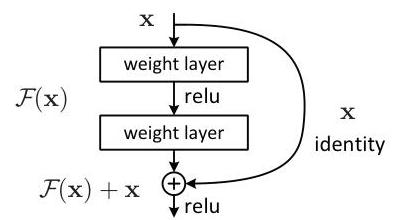
ResNet solved the fundamental observation that deeper plain networks degrade in both training and test accuracy despite having strictly greater representational capacity. The key insight is to reformulate layers as learning residual functions F(x) = H(x) - x with respect to the input, rather than learning the full mapping H(x) directly. With skip connections providing the identity shortcut, the output becomes y = F(x) + x, making it trivially easy for the network to learn identity mappings (just push F(x) toward zero) while retaining the capacity to learn complex transformations.

The residual learning framework became the default backbone architecture across computer vision and beyond. ResNet-152 achieved 3.57% top-5 error on ImageNet, and the skip connection idea proved so general that it influenced virtually every subsequent deep architecture, including transformers (where residual connections around attention and FFN sublayers are standard). ResNet remains one of the most cited papers in all of computer science.

Key Contributions

Residual learning formulation: Instead of learning H(x) directly, the network learns F(x) = H(x) - x with output y = F(x) + x, making identity mappings trivially learnable (just push weights to zero)
Bottleneck blocks: 1x1 -> 3x3 -> 1x1 convolution pattern reduces parameters while maintaining accuracy, making 50+ layer networks practical (ResNet-50 has only 25.5M parameters vs VGG-16's 138M)
Projection shortcuts: 1x1 convolutions handle dimension mismatches between input and residual when spatial size or channel count changes across stages
Scalable depth: Demonstrated consistent accuracy improvements from 18 to 152 layers, definitively showing deeper networks outperform shallower ones when gradient flow is maintained
Transfer to detection/segmentation: ResNet features improved COCO object detection by large margins, establishing residual networks as universal visual backbones

Architecture / Method

Residual learning building block with shortcut connection

Architecture comparison: VGG-19, 34-layer plain network, and 34-layer ResNet

Basic Residual Block (ResNet-18/34):
                 x
                 │
        ┌────────┤
        │        ▼
        │   ┌──────────┐
        │   │ 3x3 Conv │
        │   │ BN + ReLU│
        │   └────┬─────┘
        │        ▼
        │   ┌──────────┐
        │   │ 3x3 Conv │
        │   │ BN       │
        │   └────┬─────┘
        │        │
        └───►(+)◄┘    y = F(x) + x
              │
            ReLU
              │
              ▼
              y

Bottleneck Block (ResNet-50/101/152):
                 x
                 │
        ┌────────┤
        │        ▼
        │   ┌──────────────┐
        │   │ 1x1 Conv     │  (256 ─► 64)
        │   │ BN + ReLU    │
        │   └────┬─────────┘
        │        ▼
        │   ┌──────────────┐
        │   │ 3x3 Conv     │  (64 ─► 64)
        │   │ BN + ReLU    │
        │   └────┬─────────┘
        │        ▼
        │   ┌──────────────┐
        │   │ 1x1 Conv     │  (64 ─► 256)
        │   │ BN           │
        │   └────┬─────────┘
        │        │
        └───►(+)◄┘
              │
            ReLU
              │
              ▼

Full Network (ResNet-50 example):
┌───────┐  ┌────────┐  ┌────────┐  ┌────────┐  ┌────────┐  ┌─────┐  ┌────┐
│7x7 cv │─►│Stage 1 │─►│Stage 2 │─►│Stage 3 │─►│Stage 4 │─►│ GAP │─►│ FC │
│stride 2│  │64ch    │  │128ch   │  │256ch   │  │512ch   │  │     │  │1000│
│MaxPool │  │56x56   │  │28x28   │  │14x14   │  │7x7     │  │     │  │    │
└───────┘  │3 blocks│  │4 blocks│  │6 blocks│  │3 blocks│  └─────┘  └────┘
            └────────┘  └────────┘  └────────┘  └────────┘

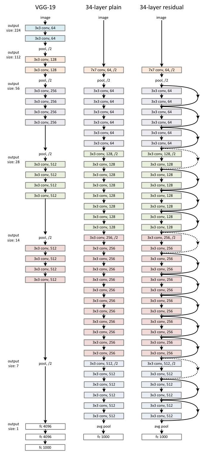
ResNet builds on the VGG philosophy of using small (3x3) convolution filters but adds shortcut connections that skip one or more layers. The basic residual block consists of two 3x3 conv layers with batch normalization and ReLU, plus an identity shortcut: y = F(x, {W_i}) + x. When input and output dimensions differ (due to stride or channel changes), a projection shortcut using 1x1 convolution is used: y = F(x, {W_i}) + W_s * x.

For deeper networks (50+ layers), bottleneck blocks are used: 1x1 conv (reduce channels from 256 to 64), 3x3 conv (64 channels), 1x1 conv (expand back to 256). This reduces computational cost by ~3x compared to two 3x3 layers while maintaining accuracy. The full architecture follows a stage-based design: conv7x7 stride 2, max pool, then 4 stages of residual blocks with progressively increasing channels (64, 128, 256, 512) and decreasing spatial resolution (56x56, 28x28, 14x14, 7x7), followed by global average pooling and a fully-connected classification layer.

Training uses SGD with momentum 0.9, weight decay 1e-4, batch size 256, and learning rate starting at 0.1 divided by 10 when error plateaus. Data augmentation includes random crops from resized images, horizontal flips, and per-pixel mean subtraction. No dropout is used (batch normalization provides sufficient regularization).

Results

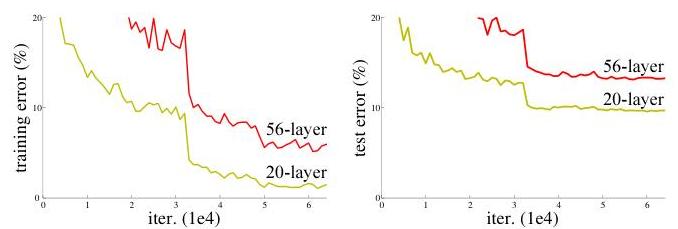
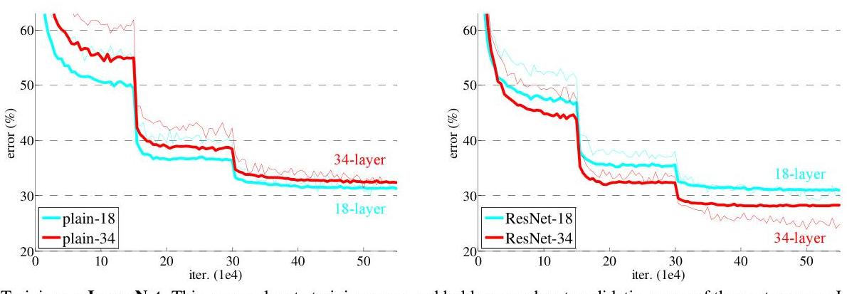
Degradation problem: deeper plain networks show higher training error

Training curves showing plain networks degrade while ResNets improve with depth

Degradation is not overfitting: 56-layer plain networks have higher training error than 20-layer plain networks on ImageNet, proving the problem is optimization difficulty, not capacity
Residual networks do not degrade with depth: ResNet-152 (21.43% top-1 error) consistently outperforms ResNet-34 (25.03% top-1 error), with monotonic improvement as layers increase; experiments successfully trained networks exceeding 1000 layers
Skip connections enable gradient flow: Gradients through a residual block have the form dL/dx = dL/dy * (1 + dF/dx), where the identity term 1 prevents vanishing gradients even when dF/dx is small
Layer response analysis: ResNets exhibit smaller, uniformly distributed responses across layers compared to plain networks, indicating superior information flow throughout the network
Generalization across tasks: Same architecture wins ImageNet classification (3.57% top-5), COCO detection, and COCO segmentation, demonstrating broad applicability
ILSVRC 2015 winner: ResNet ensemble achieved 3.57% top-5 error on the ImageNet test set, securing first place in classification, detection, and localization tracks

Limitations & Open Questions

The paper does not fully explain why plain networks degrade (optimization landscape analysis came later)
Projection shortcuts for dimension matching add parameters; the tradeoff between identity and projection shortcuts is not exhaustively explored
The optimal depth is dataset-dependent; 1000+ layer networks showed diminishing returns on ImageNet without further architectural changes (addressed in the follow-up identity mappings paper)