GPipe: Efficient Training of Giant Neural Networks using Pipeline Parallelism
Overview
GPipe introduces micro-batch pipeline parallelism as a practical method for training neural networks too large to fit on a single accelerator. The core idea is to partition a neural network into K sequential stages across K devices, then subdivide each mini-batch into M micro-batches that are pipelined through the stages. This allows multiple devices to compute simultaneously on different micro-batches, dramatically reducing the idle time that plagues naive model parallelism. Combined with activation re-materialization (recomputing forward activations during backprop instead of storing them), GPipe enables training of models that far exceed single-device memory.
As model sizes grew beyond single-GPU memory limits, naive model parallelism suffered from catastrophic idle time -- with K pipeline stages, (K-1)/K of compute is wasted as devices sit idle waiting for forward and backward passes to propagate. GPipe solves this by splitting each mini-batch into M micro-batches, reducing idle time from O(K) to O(K/M). With M=8 and K=8, efficiency jumps from 12.5% (naive) to 88.9%. The approach maintains fully synchronous gradient computation with no approximations, ensuring training dynamics are mathematically identical to single-device training.
GPipe enabled training a 557M-parameter AmoebaNet to 84.4% ImageNet accuracy, scaling AmoebaNet to 1.8B parameters across 8 accelerators (25x increase), and scaling a Transformer to 83.9B parameters across 128 accelerators (298x increase), establishing the pipeline parallelism paradigm that became foundational for training virtually all large language models. Megatron-LM, PaLM, and other large-scale training systems build directly on the principles introduced here.
Key Contributions
- Micro-batch pipeline parallelism: Split mini-batch of size B into M micro-batches of size b = B/M, pipeline them through K stages so multiple devices compute simultaneously, achieving efficiency M/(M+K-1) compared to 1/K for naive pipelining
- Gradient accumulation across micro-batches: Each device accumulates gradients from all M micro-batches before performing a single synchronized parameter update, maintaining mathematical equivalence to standard mini-batch SGD
- Re-materialization (activation checkpointing): Forward-pass activations are discarded after each micro-batch and recomputed during the backward pass, trading approximately 33% extra computation for massive memory savings
- Automatic pipeline partitioning: The model is partitioned into K sequential stages assigned to K devices, with the constraint that stages must form an acyclic sequence
- Synchronous training with exact gradients: Unlike asynchronous approaches, GPipe maintains fully synchronous gradient computation with no approximations
Architecture / Method
┌─────────────────────────────────────────────────────────────┐
│         GPipe: Micro-Batch Pipeline Parallelism              │
│                                                             │
│  Model split into K=4 stages across 4 devices:              │
│                                                             │
│  Naive Model Parallelism (wasteful):                        │
│  Time ──►                                                   │
│  Dev 1: [F1────]                    [B1────]                │
│  Dev 2:         [F2────]      [B2────]                      │
│  Dev 3:               [F3──][B3──]                          │
│  Dev 4:                [F4][B4]                              │
│         ████ = idle ("bubble")  ──► 75% idle!               │
│                                                             │
│  GPipe with M=4 micro-batches (pipelined):                  │
│  Time ──►                                                   │
│  Dev 1: [F1][F2][F3][F4]          [B4][B3][B2][B1]         │
│  Dev 2:     [F1][F2][F3][F4]  [B4][B3][B2][B1]             │
│  Dev 3:         [F1][F2][F3][F4][B4][B3][B2][B1]           │
│  Dev 4:             [F1][F2][F3][F4][B4][B3][B2][B1]       │
│                ███                                          │
│         bubble = (K-1)/(M+K-1) = 3/7 ≈ 43%                 │
│         With M=32: bubble = 3/35 ≈ 8.6%                    │
│                                                             │
│  Re-materialization:                                        │
│  Forward:  compute activations ──► discard                  │
│  Backward: recompute activations ──► compute gradients      │
│  Cost: ~33% extra compute, massive memory savings           │
│                                                             │
│  Gradient accumulation: sum grads across all M micro-batches│
│  ──► single synchronized weight update (exact SGD)          │
└─────────────────────────────────────────────────────────────┘
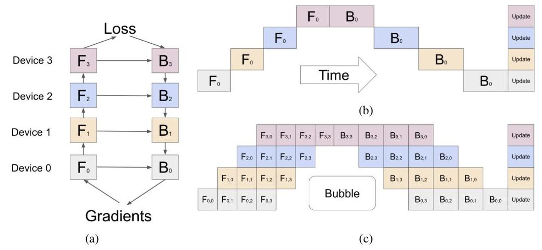
GPipe's pipeline parallelism works as follows. Consider a neural network that can be decomposed as a sequential composition of functions: f = f_K . f_{K-1} . ... . f_1. Each function f_k is assigned to device k as a "stage." During training, a mini-batch of size B is split into M micro-batches of size b = B/M.
In the forward pass, micro-batch 1 enters stage 1 on device 1. As soon as stage 1 finishes processing micro-batch 1 and passes the result to stage 2 on device 2, stage 1 immediately begins processing micro-batch 2. This creates a pipeline where, in steady state, all K devices are simultaneously processing different micro-batches at different stages. The forward pass for all M micro-batches completes after M + K - 1 time steps (compared to M * K for sequential execution).
After all forward passes complete, the backward pass proceeds in reverse order through the pipeline, with gradients flowing from stage K back to stage 1. Each device accumulates gradients across all M micro-batches before performing a single weight update, ensuring the training is mathematically equivalent to processing the entire mini-batch at once.
The pipeline "bubble" -- idle time at the start and end when not all stages have work -- costs K-1 time steps out of M+K-1 total. By making M much larger than K, this overhead becomes negligible. For M=32 and K=4, efficiency is 32/(32+3) = 91.4%.
Re-materialization addresses the memory bottleneck: rather than storing all intermediate activations from the forward pass for use in backpropagation, each micro-batch's activations are discarded after the forward pass and recomputed on-the-fly during the backward pass. This increases computation by roughly 33% (one extra forward pass) but reduces peak activation memory from O(N) to O(N/K) per device, where N is the total number of layers.
Results
| Model | Scale | Result |
|---|---|---|
| AmoebaNet (GPipe) | 557M params | 84.4% ImageNet top-1 accuracy |
| AmoebaNet (GPipe, 8 accelerators) | 1.8B params (25x increase over single accelerator) | Maximum scalable model size demonstrated |
| Transformer (GPipe, 128 partitions) | 83.9B params (298x increase over single accelerator) | Maximum scalable model size demonstrated |
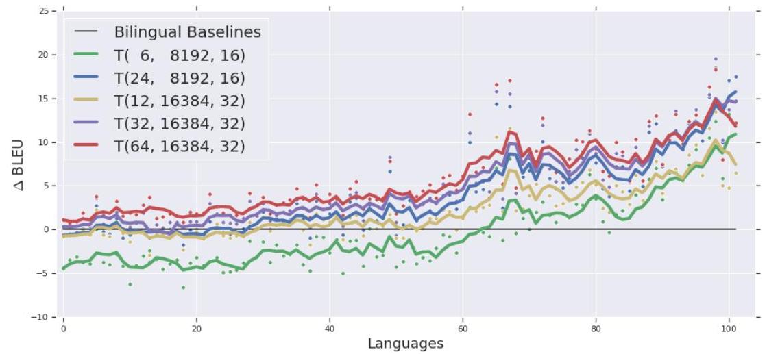
| Transformer (GPipe) | 6B params, 128-layer | Outperforms 350M bilingual models on 100 language pairs |
- Near-linear scaling: with M micro-batches and K stages, pipeline efficiency is MK / (MK + K - 1), approaching 100% as M grows; empirically demonstrated near-linear speedup on multi-accelerator setups
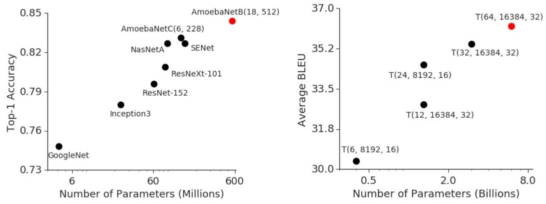
- ImageNet SOTA: 557M-parameter AmoebaNet achieves 84.4% top-1 ImageNet accuracy; on 8 accelerators GPipe scales AmoebaNet to 1.8B parameters (25x increase over a single accelerator), demonstrating that pipeline parallelism enables training models that far exceed single-device memory capacity
- Massive Transformer training: on 128 accelerators GPipe scales a Transformer to 83.9B parameters (298x increase over a single accelerator); a 6B-parameter 128-layer multilingual Transformer consistently outperforms 350M bilingual baselines across 100 language pairs
- Memory reduction: re-materialization reduces peak activation memory from O(N) to O(N/K) per device, enabling models and batch sizes that otherwise would not fit in device memory
- Training dynamics are identical to single-device training: no staleness, no gradient approximation, no learning rate adjustments needed
Limitations & Open Questions
- Pipeline bubbles still waste some compute at the start and end of each mini-batch (K-1 idle timesteps), which becomes significant when M is small relative to K
- The approach requires the model to be decomposable into sequential stages, which is less natural for architectures with skip connections, mixture-of-experts, or complex branching topologies
- Re-materialization adds approximately 33% computational overhead; more sophisticated checkpointing strategies (selective checkpointing) can reduce this but add implementation complexity