Training Compute-Optimal Large Language Models
Overview
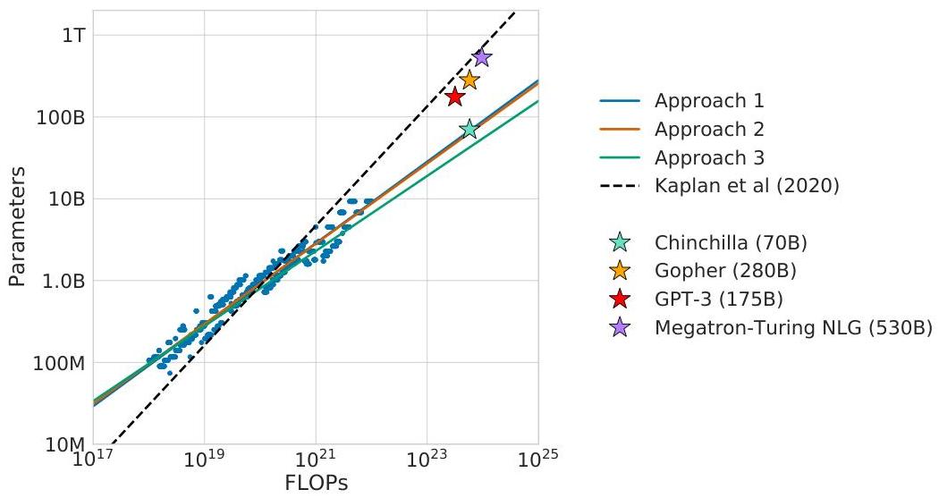
The Chinchilla paper (Hoffmann et al., DeepMind, 2022) is one of the most consequential papers in the LLM era because it corrected the field's scaling intuition. Kaplan et al. (2020) had recommended allocating most compute to model size and training for fewer steps ("train large, stop early"). Chinchilla demonstrated that this prescription was significantly suboptimal: for compute-optimal training, model parameters and training tokens should scale roughly equally. Specifically, doubling compute should be split equally between doubling parameters and doubling data.
The practical implication was stark. Many flagship models of 2021-2022 were dramatically undertrained relative to their parameter count. GPT-3 (175B parameters, 300B tokens) and Gopher (280B parameters, 300B tokens) used far fewer tokens than their compute budgets warranted. Chinchilla -- a 70B parameter model trained on 1.4T tokens using the same compute as Gopher -- outperformed Gopher on the majority of evaluation benchmarks despite being 4x smaller. This proved that the field had been wasting compute by making models too large and training them on too little data.
The paper fundamentally redirected the industry. After Chinchilla, the LLM community shifted toward training smaller models on much larger datasets (LLaMA 7B on 1T tokens, LLaMA 2 on 2T tokens), and data curation became as important as model architecture. The "Chinchilla-optimal" frontier became the standard reference point for evaluating whether a model was efficiently trained.
Key Contributions
- Corrected scaling law for compute-optimal training: Model parameters N and training tokens D should scale equally with compute budget C, not favoring N as Kaplan et al. recommended. The relationship is approximately N_opt proportional to C^0.5 and D_opt proportional to C^0.5
- Three independent estimation approaches: Used three different methods to estimate optimal N-D tradeoffs (fixing model size and varying tokens, IsoFLOP profiles, and parametric loss modeling), all converging on the same conclusion
- Chinchilla model (70B, 1.4T tokens): Trained a 70B parameter model on 1.4T tokens using the same compute as the 280B parameter Gopher, demonstrating that it outperforms Gopher on the majority of benchmarks
- Exposed widespread undertraining: Showed that GPT-3, Gopher, Jurassic-1, and Megatron-Turing NLG were all significantly undertrained -- for example, Table 3 (Approach 1) implies GPT-3 should have been trained on ~3.7T tokens (roughly 12x more) and Gopher on ~5.9T tokens (roughly 20x more) for their compute budgets
- Data becomes the bottleneck: By establishing that tokens should scale with parameters, the paper shifted attention to data collection, curation, and deduplication as critical infrastructure
Architecture / Method
     Chinchilla: Three Approaches to Compute-Optimal Scaling

  ┌──────────────────────────────────────────────────────────┐
  │  Approach 1: Fix Model Size N, Vary Data D               │
  │                                                          │
  │  Loss │\                                                 │
  │       │ \___________  ◄── diminishing returns from       │
  │       │              ──    more data at fixed N           │
  │       └──────────────────── Tokens D                     │
  │  Repeat for N = 70M, 150M, ..., 16B                      │
  ├──────────────────────────────────────────────────────────┤
  │  Approach 2: IsoFLOP Profiles (Fix Compute C)            │
  │                                                          │
  │  Loss │     *                                            │
  │       │   *   *      ◄── optimal N at each C level       │
  │       │  *     *                                         │
  │       └──────────────────── Model Size N                 │
  │  Repeat for C = 10^18, 10^19, ..., 10^21 FLOPs          │
  ├──────────────────────────────────────────────────────────┤
  │  Approach 3: Parametric Fit                              │
  │                                                          │
  │  L(N,D) = E + A/N^α + B/D^β                             │
  │  Minimize over N,D subject to C ≈ 6ND                   │
  │  ──► N_opt ∝ C^0.5,  D_opt ∝ C^0.5                     │
  └──────────────────────────────────────────────────────────┘

  All 3 converge: scale params and data equally with compute
      Gopher (280B, 300B tok) ──► Chinchilla (70B, 1.4T tok)
The study trained over 400 transformer models ranging from 70 million to 16 billion parameters on 5 to 500 billion tokens, using the same basic architecture as Gopher -- a decoder-only Transformer with standard training details (AdamW, cosine schedule, SentencePiece tokenizer). The key contribution is methodological rather than architectural: three independent approaches to estimating the compute-optimal frontier.
Approach 1 (Fix N, vary D): Train models of fixed size (70M to 16B parameters) on varying amounts of data (5B to 500B tokens) and, for each model size, observe where the loss curve bends (diminishing returns from more data). This traces out the optimal data allocation for each model size.
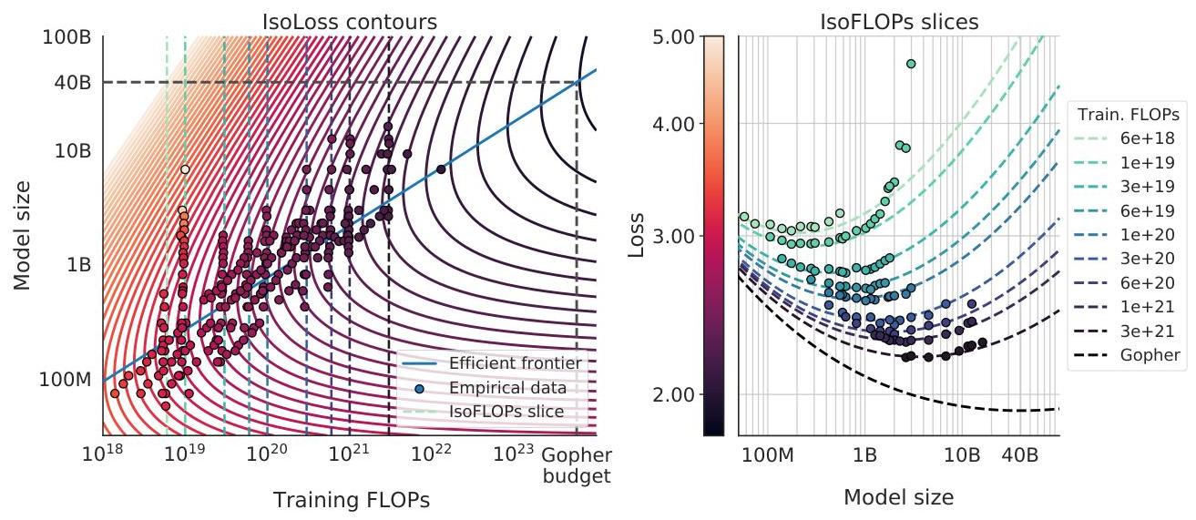
Approach 2 (IsoFLOP profiles): For a fixed compute budget, train models of varying sizes (each necessarily seeing different amounts of data since C ~ 6ND). Plot loss vs. model size for each compute level. The minimum of each curve gives the optimal model size for that compute budget. Repeating across compute budgets traces the scaling relationship.
Approach 3 (Parametric loss model): Fit L(N, D) = E + A/N^alpha + B/D^beta to the full grid of (N, D, L) observations, then analytically minimize over N and D for each compute budget C = 6ND. This yields closed-form scaling coefficients.
All three approaches converge: a = b ~ 0.5 in the relationship N_opt ~ C^a, D_opt ~ C^b, meaning parameters and data should scale equally.
Results
| Model | Params | Tokens | MMLU | Compute |
|---|---|---|---|---|
| Chinchilla | 70B | 1.4T | 67.6% | 1x (same as Gopher) |
| Gopher | 280B | 300B | 60.0% | 1x |
| GPT-3 | 175B | 300B | 43.9% | - |
- Chinchilla (70B) outperforms Gopher (280B): On the majority of evaluation tasks including MMLU (67.6% vs 60.0%), HellaSwag, LAMBADA, and others, despite being 4x smaller and using the same compute budget
- Three estimation methods agree: All three independent approaches for estimating optimal N-D allocation converge on the same scaling relationship (a ~ b ~ 0.5), providing strong evidence for the conclusion
- MMLU state-of-the-art: Chinchilla achieved 67.6% on MMLU, surpassing Gopher (60.0%), GPT-3 (43.9%), and all other models at the time of publication. Also demonstrated lower perplexity and superior performance on HellaSwag, LAMBADA, and other downstream tasks
- Inference efficiency: As a 4x smaller model, Chinchilla is substantially cheaper and faster at inference time, providing both better quality and lower deployment cost
- Existing models are an order of magnitude undertrained: Analysis shows GPT-3 (175B) should have been trained on ~3.7T tokens (vs 300B actual, ~12x more) and Gopher (280B) on ~5.9T tokens (vs 300B actual, ~20x more) for their compute budgets (Table 3, Approach 1 estimates)
Limitations & Open Questions
- The study uses only autoregressive Transformer LMs on English text; whether the a ~ b ~ 0.5 relationship holds for other architectures (encoder-decoder, state-space models), modalities (vision, multimodal), or languages is not established
- The scaling law describes training loss, not downstream task performance; a compute-optimal model for loss may not be compute-optimal for specific capabilities, emergent behaviors, or safety properties
- The paper does not account for inference cost: a smaller model trained on more data is cheaper to deploy, suggesting that the true optimum for practical systems should weight inference cost, shifting the allocation further toward smaller models with even more data (as argued by LLaMA)
Connections
- Scaling Laws For Neural Language Models -- Kaplan et al. scaling laws that Chinchilla corrected
- Language Models Are Few Shot Learners -- GPT-3, shown to be significantly undertrained by Chinchilla analysis
- Attention Is All You Need -- Transformer architecture used throughout
- Gpipe Easy Scaling With Micro Batch Pipeline Parallelism -- pipeline parallelism for training large models
- Foundation Models -- broader context on foundation model scaling
- Machine Learning -- general ML concepts