GaussianLSS: Toward Real-world BEV Perception with Depth Uncertainty via Gaussian Splatting
Overview
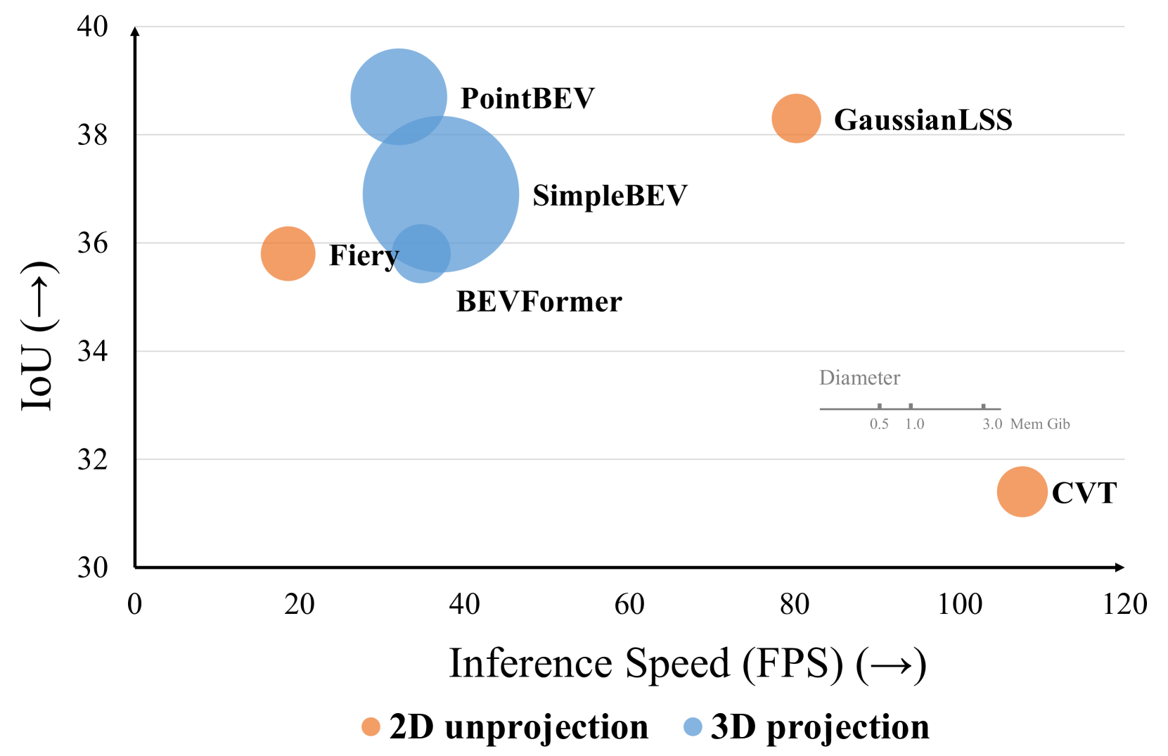
Bird's-Eye View (BEV) perception faces a fundamental trade-off between accuracy and computational efficiency. High-performing 3D projection methods like BEVFormer achieve excellent results but require substantial compute, while efficient 2D unprojection methods like Lift-Splat-Shoot (LSS) struggle with depth ambiguity and robustness. GaussianLSS bridges this gap by incorporating explicit depth uncertainty modeling within the efficient LSS unprojection framework, adapted through Gaussian Splatting.
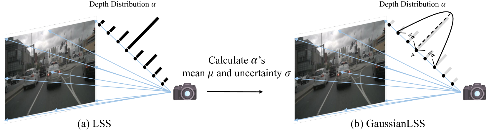
The core innovation is treating depth estimation as a probabilistic problem rather than a deterministic one. For each pixel, the network predicts not just a depth value but a full depth distribution, from which both a mean depth and variance (uncertainty) are computed. This 1D depth uncertainty is transformed into a full 3D Gaussian representation with mean and covariance, then projected onto the BEV plane via a novel Gaussian Splatting aggregation that produces dense, uncertainty-aware BEV features.
GaussianLSS achieves 38.3% IoU for vehicle BEV segmentation -- within 0.4% of the state-of-the-art 3D projection method PointBEV (38.7%) -- while running at 80.2 FPS (2.5x faster) and using only 0.33 GiB memory (3.8x less). This makes it a practical choice for real-world deployment in resource-constrained autonomous vehicles where both accuracy and efficiency matter.
Key Contributions
- Explicit depth uncertainty modeling: Predicts depth distributions per pixel and computes mean and variance, quantifying confidence in depth estimates rather than producing point estimates
- 3D uncertainty transformation: Converts 1D depth uncertainty into full 3D Gaussian representations (mean + covariance) through camera geometry unprojection
- Gaussian Splatting for BEV aggregation: Adapts Gaussian Splatting from radiance field rendering to BEV perception, using uncertainty-aware 3D Gaussians for efficient feature projection
- Multi-scale BEV rendering: Projects Gaussians onto BEV planes at multiple resolutions (50x50, 100x100, 200x200) to mitigate distortions from inconsistent depth estimates
- Accuracy-efficiency balance: Achieves near-SOTA accuracy at 2.5x speed and 3.8x memory savings compared to 3D projection methods
Architecture / Method
┌──────────────────────────────────────────────────────────────────┐
│                     GaussianLSS Pipeline                          │
│                                                                   │
│  ┌──────────┐    ┌───────────┐    ┌──────────────────────────┐    │
│  │ Multi-cam │───►│ Backbone  │───►│ CNN Head (per pixel)     │    │
│  │ Images    │    │           │    │  ├─ F_i  (features)      │    │
│  └──────────┘    └───────────┘    │  ├─ α_i  (opacity)       │    │
│                                   │  └─ P_i  (depth distrib) │    │
│                                   └────────────┬─────────────┘    │
│                                                │                  │
│                         ┌──────────────────────▼───────────────┐  │
│                         │  Depth Uncertainty Modeling           │  │
│                         │  μ = Σ P_i · d_i                     │  │
│                         │  σ² = Σ P_i · (d_i - μ)²            │  │
│                         │  Soft range: [μ-kσ, μ+kσ]           │  │
│                         └──────────────────────┬───────────────┘  │
│                                                │                  │
│                         ┌──────────────────────▼───────────────┐  │
│                         │  3D Uncertainty Transformation        │  │
│                         │  Unproject via intrinsics (I)         │  │
│                         │  + extrinsics (E) ──►                 │  │
│                         │  3D Gaussian (μ_3d, Σ)                │  │
│                         └──────────────────────┬───────────────┘  │
│                                                │                  │
│                    g_i = (μ_3d, Σ, F_i, α_i)   │                  │
│                                                │                  │
│                         ┌──────────────────────▼───────────────┐  │
│                         │  Multi-scale BEV Gaussian Splatting   │  │
│                         │  Project onto BEV at 50/100/200 res   │  │
│                         │  F_BEV(x) = Σ F_i · α_i · G_i(x)    │  │
│                         │  (80% Gaussians filtered by opacity)  │  │
│                         └──────────────────────┬───────────────┘  │
│                                                │                  │
│                         ┌──────────────────────▼───────────────┐  │
│                         │  BEV Decoder ──► Segmentation Map     │  │
│                         └──────────────────────────────────────┘  │
└──────────────────────────────────────────────────────────────────┘
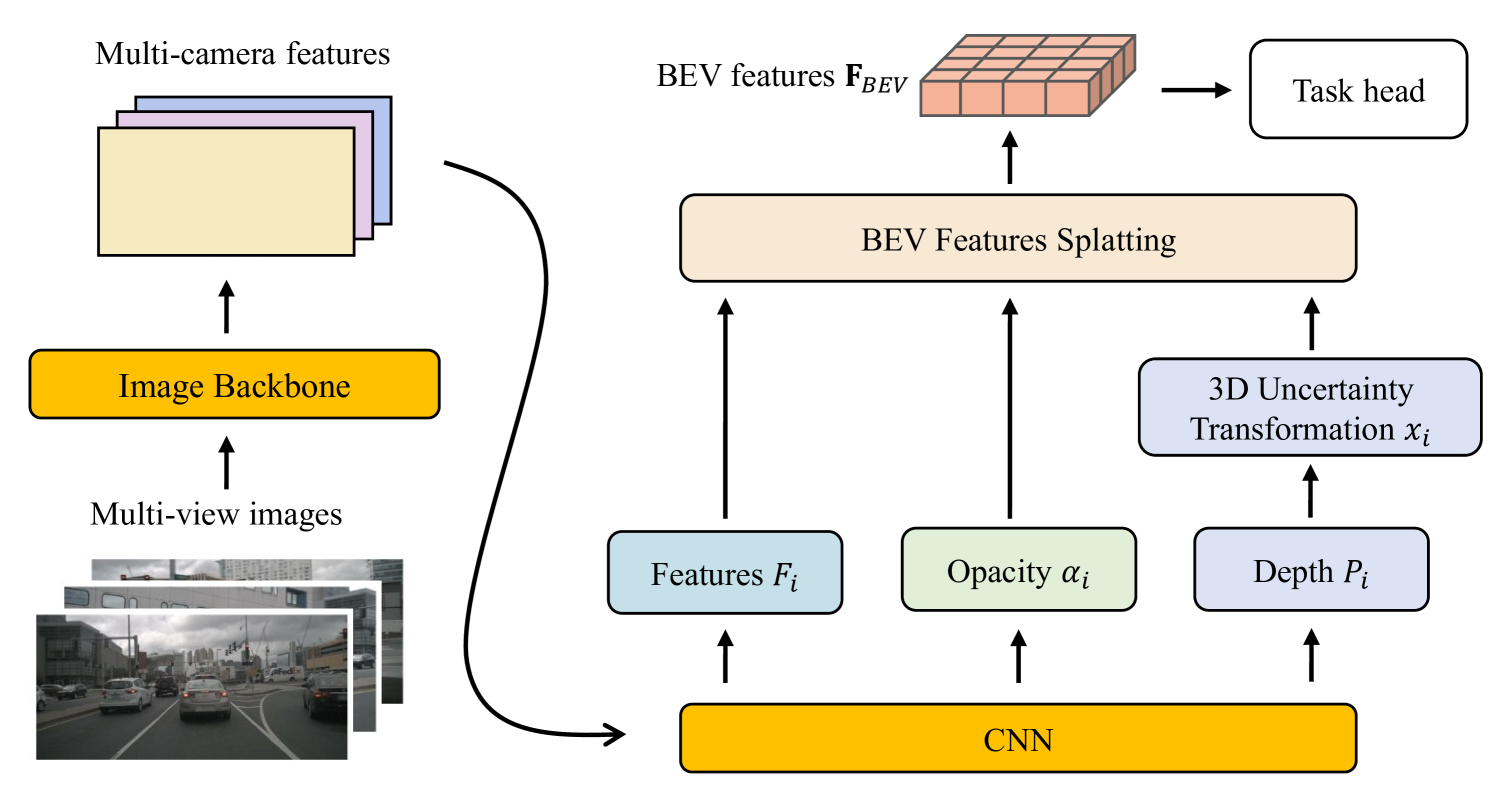
The framework processes multi-view images through a backbone network to extract features, then a CNN layer outputs three components per pixel: splatting features (F_i), opacity values (alpha_i), and depth distributions (P_i).
Depth Uncertainty Modeling: For each pixel, a soft depth mean and variance are computed from the predicted distribution:
- mu = sum(P_i * d_i) (expected depth)
- sigma^2 = sum(P_i * (d_i - mu)^2) (depth uncertainty)
A soft depth range [mu - k*sigma, mu + k*sigma] adapts to estimated uncertainty, where k is an error tolerance coefficient.
3D Uncertainty Transformation: The soft depth range is unprojected into 3D space using camera intrinsics (I) and extrinsics (E), producing a 3D Gaussian with mean mu_3d and covariance Sigma that represents the spatial uncertainty ellipsoid for each pixel's depth estimate.
Gaussian Splatting Aggregation: Each pixel's 3D Gaussian (mu_3d, Sigma), splatting features (F_i), and opacity (alpha_i) form a complete 3D Gaussian primitive: g_i = (mu_3d, Sigma, F_i, alpha_i). These are projected onto the BEV plane via alpha-blending: F_BEV(x) = sum(F_i * alpha_i * G_i(x)). An opacity-based filtering (80% of Gaussians have opacity < 0.01) acts as an automatic semantic filter.
Results
| Method | Type | Vehicle IoU | Pedestrian IoU | FPS | Memory (GiB) |
|---|---|---|---|---|---|
| LSS | 2D unproj | 32.1 | 15.0 | — | — |
| SimpleBEV | 2D unproj | 36.9 | 17.1 | 37.1 | 3.31 |
| BEVFormer | 3D proj | 35.8 | 16.4 | 34.7 | 0.47 |
| PointBEV | 3D proj | 38.7 | 18.5 | 32.0 | 1.26 |
| GaussianLSS | 2D unproj | 38.3 | 18.0 | 80.2 | 0.33 |
GaussianLSS outperforms all 2D unprojection methods and comes within 0.4% IoU of PointBEV for vehicles (38.3% vs 38.7%) while being 2.5x faster and using 3.8x less memory. For pedestrian segmentation, it achieves 18.0% IoU, trailing PointBEV (18.5%) by only 0.5%. It particularly excels at long-range objects (beyond 30m), where depth uncertainty is naturally higher and explicit uncertainty modeling provides 1.3% IoU improvement over methods using fixed spatial extents.
Limitations & Open Questions
- Single-frame only: No temporal fusion across frames; incorporating temporal depth uncertainty could further improve accuracy and stability
- nuScenes only: Evaluation limited to nuScenes; robustness across diverse driving domains (rain, night, different camera setups) is untested
- Gaussian Splatting overhead: While efficient overall, the Gaussian representation adds complexity compared to the simple LSS pillar pooling; engineering optimization for production deployment is needed
Connections
- Directly extends Lift Splat Shoot Encoding Images From Arbitrary Camera Rigs By Implicitly Unprojecting To 3D (LSS) with uncertainty-aware depth and Gaussian Splatting aggregation
- Addresses efficiency limitations of Bevformer Learning Birds Eye View Representation From Multi Camera Images Via Spatiotemporal Transformers (BEVFormer) while approaching its accuracy
- BEV features produced by GaussianLSS could serve as input to end-to-end planners like Planning Oriented Autonomous Driving (UniAD) or Vad Vectorized Scene Representation For Efficient Autonomous Driving (VAD)
- Evaluated on Nuscenes A Multimodal Dataset For Autonomous Driving (nuScenes) benchmark